Geospatial analysis report · Oregon Cascades, USA

Vegetation, moisture and canopy height in a mountain forest

Three open data sources, eight scripts and one web page. The analysis measures how greenness (NDVI), leaf water content (NDMI) and canopy height (LiDAR) change with elevation, inside two coniferous-forest watersheds.

The question

Does the forest change as the mountain rises?

Satellite imagery and a LiDAR survey can measure a forest without setting foot in it. The project covers the whole workflow: downloading the data, computing the indices, delineating the watersheds, comparing interpolation methods and publishing the result, using only free software.

Greenness does not fall steadily with elevation. In almost every elevation band NDVI stays between –, but in the – band it drops to –. NDMI nearly halves: – against –. That is why the overall correlation with elevation is weak (−0.21): a straight line cannot describe a localized drop.

The walkthrough

From satellite to analysis zones

Scroll: the map changes layer with each step. You can also pick a layer with the buttons.

The area and its two watersheds

A box of about 4.8 × 4.4 km with strong relief. From the elevation model I computed where the water flows, which gave 2 watersheds of – km². Together they cover about 87 % of the box.

A diagonal ridge separates the two. The straight edges are the limit of the downloaded area: the real watersheds continue beyond it.

Tool: pysheds (flow direction and accumulation) · Copernicus DEM GLO-30

How green: NDVI

Healthy leaves absorb red light and reflect a lot of near-infrared. NDVI condenses that into one number: close to 1 means dense forest. It was computed from 81 Sentinel-2 scenes from 2025 with under 40 % cloud, discarding clouds and shadows with the scene classification, and averaged over July to September.

Forest dominates the map (median 0.85), but there are red patches with straight edges. They look like clear-cuts; that is a hypothesis this analysis does not confirm.

Tool: pystac-client · odc-stac · xarray · rioxarray

How much water in the leaf: NDMI

It swaps red for shortwave infrared, which water absorbs. It is an indicator of water in vegetation, not a measure of soil moisture.

It follows the same pattern as NDVI, with more contrast inside the forest: it runs from −0.41 to 0.62.

Tool: the same Sentinel-2 bands · SCL mask

How tall the trees are: LiDAR

An aircraft maps the terrain with laser pulses. With PDAL I removed noise, classified the ground and computed each point's height above it. Trees become the maximum height per cell (CHM), and bare terrain becomes the DTM.

Mind the dates: the LiDAR is from 2021 and Sentinel-2 from 2025. In the lowest-NDVI band the 2021 mean canopy is – m, the same as elsewhere: the forest was there when the aircraft flew.

Tool: PDAL (readers.ept · SMRF · hag_nn · writers.gdal) · USGS 3DEP

Analysis zones: elevation bands

To compare fairly, the watersheds were split into 150 m elevation bands and everything was summarized in each. The – band is the one that breaks the pattern: NDVI –, NDMI –.

Dashed bands have fewer than 500 pixels: their averages are unreliable.

Tool: rasterio · geopandas · DuckDB
How it was done

Eight steps, in this order

Each step is a script that reads config.yml and writes to data/processed/. Order matters: each one uses what the previous one produced.

  1. Sentinel-2: vegetation indices

    Searches the STAC catalog for scenes, reads only the 4 needed bands over the study area, masks clouds and computes NDVI and NDMI per date. It ends with a control pixel recomputed by hand.

    in: Earth Search catalog → out: ndvi_summer.tif · ndmi_summer.tif · monthly series (Zarr)

  2. Elevation model

    Downloads the Copernicus DEM tile (30 m) and reprojects it to meters.

    in: cop-dem-glo-30 → out: dem_utm.tif

  3. LiDAR with PDAL

    Five chained pipelines: download, ground classification, a sample for viewing, CHM and DTM.

    in: USGS 3DEP point cloud → out: chm.tif · dtm.tif · sample .laz

  4. Hydrology

    Fills DEM sinks, computes where water flows and how much accumulates, and delineates the watersheds and the drainage network.

    in: dem_utm.tif → out: watersheds · drainage network · 150 m bands (GeoPackage)

  5. Geostatistics in R

    Takes 300 NDMI points as if they were sensors, holds out 20 %, fits a variogram and compares kriging, IDW and Thiessen polygons.

    in: ndmi_summer.tif → out: interpolated maps · uncertainty · metrics

  6. Review in QGIS and CloudCompare

    Difference maps to see where the interpolation fails, and a point-cloud profile to check that the ground ended up under the forest.

    in: all layers → out: visual review

  7. Pixel table and SQL queries

    Joins NDVI, NDMI, elevation, canopy height and band into a 20 m GeoParquet table and summarizes it with DuckDB.

    in: all rasters → out: pixels.parquet · summary by band

  8. This page

    Converts rasters to PNG and vectors to GeoJSON, then draws the map with Leaflet and the charts as SVG.

    in: results → out: docs/

Results by band

The drop is in one band, not along a slope

Each bar is a 150 m elevation band. Highlighted: the lowest-NDVI band among those with enough data; hatched: bands with fewer than 500 pixels.

Mean NDVI

Greenness. From 0 to 1.

Mean NDMI

Leaf water content. From 0 to 1.

Canopy height

Mean height (bar) and 95th percentile (mark), in meters. LiDAR from 2021, 3 m cells.

Greenness dropped; the trees did not

In the lowest-NDVI band, the mean canopy measured in 2021 is – m, the same as in the other bands. When the aircraft flew, the forest was there.

The most likely explanation is that the greenness was lost afterwards, through clear-cutting or another disturbance. That is a hypothesis: confirming it would take imagery from several years.

Heights depend on cell size: with 3 m cells they come out taller than with 1.5 m cells, because each cell keeps the highest point over a larger surface.

View the data as a table

Interpolation

Kriging wins, but only just

300 NDMI pixels were sampled as if they were field sensors and 20 % were held out for scoring. Since the true map exists, each method's error can be measured on the 60 points none of them saw.

Error on the test points

RMSE (lower is better)

Kriging beats IDW by 2 %: with 60 test points, that gap could be chance. Thiessen, which copies the nearest sensor, is clearly worse.

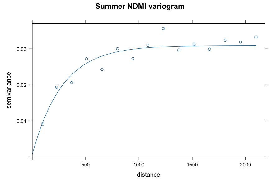
Variogram of summer NDMI: semivariance rises up to about 600 meters and levels off near 0.03

Exponential variogram: range of 282 m. Moran's I = 0.51, so nearby pixels resemble each other and interpolating is worthwhile.

Scope

What this analysis cannot claim

Showing the limits is part of the result.

  • It does not explain the cause. It shows that something changes between 900 and 1,050 m, not why. The clear-cut hypothesis is unconfirmed: it would take a multi-year image series or harvest maps.
  • The kriging points are not real sensors. They were sampled from the satellite NDMI itself, so the exercise validates the method, not field measurement.
  • NDMI is not soil moisture. It measures water in vegetation.
  • Different dates. LiDAR from 2021 and Sentinel-2 from 2025: where things changed between them, the layers do not describe the same forest.
  • Few pixels in some bands. The extreme bands give unstable averages.
  • Clipped watersheds. They end at the edge of the downloaded area, not at their natural outlet.
  • The DEM includes the canopy. It sits about 23 m above the true LiDAR terrain, which can shift the drainage network slightly.

Logbook

What went wrong and how it was fixed

Six real problems from running on real data. None of them crashed the program; most would have produced plausible but wrong results.

ProblemCauseHow it was found and fixed
Summer NDVI equal to 1.000The catalog declares an offset of −1000 in the values, but the data no longer carry it. Subtracting it left negative reflectance.The control pixel recomputed by hand gave −5.03 versus 1.000. The real value range was measured (red min. 196) and the offset was set to 0.
Credentials error reading the DEMThe file sits in a public AWS bucket, but GDAL tried to sign the request.The file was requested anonymously, without signing.
LiDAR: 177 million points and a PDAL failureThe requested resolution pulled almost all the density; PDAL runs a single output per pipeline and the ground filter fails if return numbers are 0.The point count per resolution was measured, the process was split into five stages and the return numbers were fixed.
The DEM sits 23 m above the terrainCopernicus GLO-30 is a surface model: it includes the canopy.Compared with the LiDAR DTM (correlation 0.994) and the limit was documented. For the NDVI correlation it makes no difference.
Only one watershed, 47 % of the areaThe script picked a single outlet, the one with the highest accumulation.Spotted on the map. Added n_basins; there are now two, covering 87 %.
Low-NDVI pixels with tall treesThe LiDAR is from 2021 and the NDVI from 2025.Not fixed: documented. In the lowest-NDVI band the 2021 canopy measures – m, as in the others, which points to cover lost after 2021 (unconfirmed hypothesis).

Tools

All free software

Python

  • pystac-client · odc-stac
  • xarray · rioxarray · zarr
  • rasterio · geopandas · shapely
  • pysheds · scipy
  • pyarrow · DuckDB
  • pytest · matplotlib

Data and processing

  • PDAL (point clouds)
  • R: terra · sf · gstat · spdep
  • GeoParquet · COG · Zarr
  • STAC (Earth Search)
  • conda-forge

Review and publishing

  • QGIS 4
  • CloudCompare
  • Leaflet
  • Hand-written SVG for the charts

To reproduce it

mamba env create -f environment.yml
mamba activate basins
python -m pytest tests -q          # 7 tests on synthetic data
python scripts/01_sentinel2.py     # then 02, 03 and 04 (hydrology)
Rscript scripts/05_kriging.R
python scripts/06_duckdb_summary.py
python scripts/07_web_report.py